Excel model

Information about cell protection

Valuatum Excel model includes cell protection system. Its purpose is to prevent analysts from making unintentional mistakes. Such mistakes typically cause that numbers in the Excel model do not correspond to the numbers in the web pages or that when the model is upgraded to a new version, something is lost during the process.

What is allowed, what is not?

You are allowed to

• Change the content of the cells with blue font (either with grey or white background) in the input sheets. These cells are called ‘input cells’.
• Add and remove your own sheets.
• Change the content of User’s own area in I-divQ and I-main sheets.

You are NOT allowed to

• Remove or add rows or columns in the input sheets.
• Remove or add cells in the input sheets.
• Change the content of the cells with black font in the input sheets. These are called ‘output cells’.

Cell protection prevents me doing certain things – what to do?

If you feel that the cell protection prevents you doing things that you should be able to do, please consider the instructions below. It may well be that there is another solution.

Own sheets

You are allowed to maintain your own sheets and do whatever you want with them. Own sheets are typically good for preparing your final estimates.

User’s own areas

The sheets I-divQ and I-main contain cells that are called User’s own areas. They are located on the right hand side of the estimate area. You are allowed to change the content of these cells.

Estimating with correct estimate parameters

Sometimes you may feel that you should change a formula in a cell with black font. The cell protection naturally prevents this. However, the model should always provide you a way how to handle these kinds of situations using correct estimate parameters. Here we show you two examples.

• Goodwil
  • Your intention: Change the first estimate year goodwill by adding 100 to the current value.
  • Estimate parameters for goodwill: goodwill t0 = goodwill t-1 + impairment charges + gross investments into goodwill.
  • Solution: Based on the formula it is easy to see that you should add 100 to the ‘gross investments into goodwill’ in the balance sheet estimate parameters section.
• Interest-bearing debt
  • Your intention: The model is showing too low value for interest-bearing debt in your opinion. You would like to have more interest-bearing debt (either long- or short-term).
  • Estimate parameters for interest-bearing debt: The model automatically adjusts cash and interest-bearing debt based on your estimates so that assest and liabilities always equal for estimate years. However, for debt you can define the minimum level that is always remained even thought the company’s profitability would be good.
  • Solution: Increase minimum long- or short-term debt in the balance sheet estimate parameters section.

Other solutions

In case the solutions above do not help you, you can always contact Valuatum. We are probably able to help you in using the valuation model in a proper way.

Disabling cell protection

If you for some reason need to disable cell protection (have you read the instructions above?), you can do it either temporarily or temporarily.

Please remember that if you disable cell protection, Valuatum does not quarantee the correct behaviour of the model!

Temporary disabling

You have two to disable cell protection temporarily:

1. Click Options button in the top of I-main sheet. Choose Cell Protection – Off and click Ok.
2. When you try to change a cell that you are not allowed to change, the model gives you an error message. The message also contains a button that you can use for disabling the cell protection.

When you close the model and open it again, the cell protection is automatically activated.

Permanent disabling

If you want to disable cell protection so that it is not activated when the model is re-opened, do the following:

• Click Options button in the top of I-main sheet. Choose Cell Protection – Always off and click Ok.

Automatic calculation of quarterly estimates for next year

At the end of the year, the next year quarterly estimates can be automatically calculated using a macro. In order to run the macro, do the following:

 1. Select “Generate next year Q estimates” from the drop-down menu in the upper left corner of the I-divQ -sheet.
 2. Press “Run macro”.

Calculation of Net sales and EBIT

The macro calculates seasonal variation percentages to the tables on the right side of “User’s own area”. The absolute quarterly Net sales and EBIT are then calculated based on these percentages.

Please note

• The seasonal variation estimates are based on the variation of only two previous years and are easily affected by considerable one-time variation in the figures.
• You should always critically assess the validity of the automatically created estimates and also change them to account for possible new development in the company’s operations.

Calculation of items in the income statement

The following items in the income statement are calculated by allocating the whole-year estimate evenly to the quarters:

• Other operating income
• Depreciation (tangible, intangible)
• Impairment charges
• Share of profits in associated companies
• Net financials
• Other items
• Minority interest
• Extraordinaries

The item Taxes is calculated by multiplying the quarterly Pre-tax profit with the full year tax rate from the I-main sheet.

Advanced Excel information

This page offers answers for some Excel related advanced questions.

Index

Sheets

•  What does “IO-sheets are mirror sheets of I-sheets” mean?
•  Why are the O-sheets not directly linked to the I-sheets?
•  What is the Database-interface sheet?

Function of the model

•  Why iterations is used?
•  How iterations is used?

Parameter estimation

•  Financial items

Macros

•  Year Change – what does it do exactly?
•  How does the macro ‘FixInterestExpenses’ work?
•  What does the conversion macro do?

Sheets

What does “IO-sheets are mirror sheets of I-sheets” mean?

It means that IO-sheets include the same information as I-sheets. The information comes with VLOOKUP functions on the basis of row (index number) and column (year/quarter).
(See the following question for more info.)

Why are the O-sheets not directly linked to the I-sheets?

The reason is year change operation. When you run the YearChange macro, it removes in the I-sheets the latest year and adds one estimate year so that the model would stay similar year after year.
In O-sheets it is reasonable to assume that there is one column that always refers to the current (ongoing) year. Now when there are columns removed in the I-sheets, direct links in an O-sheet would mean that columns would not change year.
However, when we use IO-sheets in between, we can always have the current year in a same column in the O-sheets.

What is Database-interface sheet?

Database-interface is a sheet where all the input figures are collected from the IO-sheets (originally from the I-sheets).

(Input figures are such figures that a user must enter him/herself, i.e. the model cannot calculate them using other figures. An example: net sales is an input figure, ROE % is an output figure, since it is calculated on the basis of the other parameters.)

The input figures continue from the Database-interface sheet to the Valuatum Database when a user starts a macro called DBUpdate. When the update process finishes, all the customers can see the model in ValuModels.

Function of the model

Why iteration is used?

When income statement and balance sheet are estimated, there is always a problem with a loop:
Interest expenses are estimated with a parameter that checks debt, debt depends on the balance sheet total, balance sheet total depends on equity, equity depends on earnings, and earnings depend on interest expenses.
Iteration must be used so that the model would work even with this loop.

How iteration is used?

Iteration can be set from the menu: Tools – Options – Calculation – Iteration. There you can define the rules for the iteration.
If there is an error inside of the loop (like always in the beginning when you start filling an empty model), the iteration does not work anymore. The problem can however be solved using FixInterestExpenses macro.

Parameter estimation

Financial items

In the I-divQ sheet net financials are estimated quarterly. Thereby sub items cannot be estimated in the sheet (we have concluded with the analysts that sub items are not relevant at quarter-level).

In the I-main sheet you also have financial items for the current year, but they are divided into the four sub items. Since we have different accuracy (in I-divQ only “net financial” items and in I-main the sub items) in different sheets, we have to make sure that there is consistency in the estimates at different levels.

Therefore we have taken the sum of quarterly net financial items and subtracted from it the three net financials sub items in I-main. These sub-items are: “Other financial expenses”, “Exchange rate differences” and “Financial income” (so all the sub items except “Interest expenses”). The result of this computation is presented in an OUTPUT figure “Interest expenses” in the I-main sheet.

Why this kind of arrangement?

Well, for the user everything is now fairly simple: If (s)he does not want to go into details, (s)he can only estimate the quarterly net financials and does not have to do anything in I-main. In this case the value in I-divQ is totally allocated to interest expenses, which is probably not so bad assumption.

If the analyst would like to estimate net financials in sub items in whole year level (as (s)he normally does with big companies), then it is also possible. It is even quite handy as the quarterly and whole year estimates go automatically hand in hand: If you change net financial estimates in I-divQ, then also the estimates in I-main change automatically. For example, if you change financial income estimates in I-main, then your interest expenses item in I-main decreases automatically to ensure that estimates in I-divQ and I-main are consistent. Of course the automatic decrease in interest expenses in I-main might be something that the analyst would not like to do, but as the items are side by side, it is easy to notice and also very easy to change back by adjusting the net financials in I-divQ. If this kind of connection would not be there, then the estimates would be easier different in different sheets.

Another possibilities would be that we would have one of these:
1.    Net financials would be split to sub-items also in quarterly estimates. This would mean 16 different values to estimate.
2.    Net financials would be only net financials also on whole year level (without sub-items: int. expenses, fin. income etc.).
3.    The consistency of different estimates (quarter level and whole year level) would be manually done. Then there would always be a great danger of human mistakes and inconsistency.

Macros

Year Change – what does it do exactly?

YearChange macro have to be run so that the structure of the model remains same year after year (current year stays in the same column etc.).

All the changes are done in the I-sheets. The following things are to be done:
1.    At first the macro inserts new columns and thus adds new estimate year to the end of the current estimate period.
2.    Then the macro copies formulas to the added columns.
3.    Since the first year will be removed in both I-sheets, all the links to these cells will be destroyed. In order to remain the values (and avoid #REF), macro first copies cells and then makes ‘paste as values’ to the same cells.
4.    There are many places in the model where in one cell there is a formula and in the following cell (year) there is an input figure (or the opposite). These limiting places have to be fixed to correspond the new lay-out: the macro copies and pastes formulas in these kind of cells.
5.    The macro also runs the FixInterestExpenses macro since the year change causes a problem in the loop.
6.    At the end the YearChange macro removes cells in the left and so the latest history year is removed in every I-sheet.
If you now have to do the year change in practice, please follow the Year change instructions.

How does the macro ‘FixInterestExpenses’ work?

At first the macro sets values in interest expenses and financial income to be zero. This is done for the first problematic year. The operation fixes the year in question.
Then the formulas are copied from the following year to the first problematic year. This does not cause the error any more.
Then all the following estimate years are set to be zero, which removes the errors from those years. After that the formulas are copied from the first problematic year to the rest of the years and now the loop has been started again.

What does the conversion macro do?

Conversion macro is used when the latest version of the empty model is wanted to adopt. The macro has been developed so that it can convert in the same run as many excel models as wanted. All the user has to do is to point the empty model and the models to be converted.

The macro is quite big and it is not reasonable to explain too detailed its operation. Basically the macro copies all the input values from the old model to the empty model. This way the empty model is sort of built again. The formatting is also copied as much as possible. In the macro there are also some special properties like recognizing of quarter and read-only. These affect to the actions taken by the macro.

At the end of the macro the old model is closed and the empty model is saved as the name of the old model. If more than one file was chosen in the beginning, the macro starts to operate with the next model.

While macro updates the old models, it creates a log file. From the file you can see whether the conversion has succeeded, how much the fair value has changed and what is the difference of the new DCF and EVA fair values.

Each model takes about 20 seconds to be converted. The time depends mostly on the saving time used (local disk is naturally faster than network drive).

Excel Model Update (Conversion)

What, when & why?

Updating your Excel model means that you update the model structure (formulas, macros, etc.) to the latest version available. (In this case it does not mean same as for example updating numbers in the model or updating numbers to the database.) After update you will have the same numbers as before but the latest properties. The changes we do to the model may be for example:

•  Change in an output sheet or a new output sheet.
•  Change in a formula (e.g. another way to calculate a key figure).
•  New estimate variable.
•  Change in macros or a new macro that offers a new property.

It is recommended to update the model regurlarly so that possible errors in the model will get fixed and you will get the latest properties. You can consider Valuatum Excel model as a program that requires updating same way as any other program.

One reason to update is that occasionally we make changes to the model formulas, we may for example add new estimate parameters. If you don’t update your Excel model, these changes won’t be available for you.

If you notice differences in the numbers in your Excel model and numbers in the web pages, the first thing you should do is to update the model and then upload the numbers to the database again.

How to update Excel model(s)?

You have two ways to update your Excel model(s):

1. Download your data to the latest model version

When to use?
This option is possible to use if

•  you don’t have any own sheets in the model,
•  you don’t have any links to external workbooks,
•  you haven’t used User’s own areas in the model.

So basically you can use this option if you have just the data in your model and you haven’t done much of customizing.

Pros and cons

+ Updating is quick and simple (just download the data to the latest model).
+ Error risk is smaller (the second option may have problems with old models).
– The new model will contain only the basic data; e.g. external links will disappear.

Instructions:
1.    Download the latest model version (latest empty model):

• Go to the system’s Analyst section.
• Click Excel files button.
• Download the latest empty model to your computer.

2.    Open the empty model in your computer.
3.    Run DB2Excel and select your company from the list.
4.    Save the file with another name.

As a result you will have the latest model version including the same estimates as you have currently in the database.

2. Convert your old model to the latest model version

When to use?
This option is recommended if

•  you have added own sheets to the model,
•  you have links to external workbooks,
•  you have used User’s own areas in the model,
•  you have added many user comments to the model.

Compared to the first update option this option is needed when you have a lot of your own changes that you would like to remain in the new version too.

One good reason to use this option is that it enables updating multiple models at once. It also gives you a possibility to easily check if numbers have changed during the update.

Pros and cons

+ Your own properties (external links, own sheets, etc.) will remain in the new model.
+ You can update multiple models at once..
+ You can easily compare the old and new values using O-compare sheet.
– The process is a bit more complicated than in the first option.
– If you have a very old model, the conversion macro may not be able to update it properly.

Instructions:
1.    Download the latest model version (latest empty model) and the latest conversion macro:

• Go to the system’s Analyst section.
• Click Excel files button.
• Download the latest empty model to your computer.
• Download the latest conversion macro to your computer.

2.    Create a backup copy of your model(s).
3.    Open the conversion macro in your computer and close all other Excel files.
4.    Run the macro by clicking the button.
5.    First choose the empty model.
6.    Then choose the model(s) you would like to update.
7.    Finally set 0’s to the waiting questions (0 h 0 min, i.e. start immediately).

The macro goes through each model one by one and copies the input values to the empty model. After the process has finished, you have models with the latest properties.

The process takes time about 20-40 seconds per file depending on the computer efficiency. Thus updating 10 models takes about 5 minutes.

After the update you are able to compare possible changes in the values in O-compare sheet. This sheet will appear during the update and you can remove it after you don’t need it anymore. If you notice some significant changes in the values, you should compare the old and new version more detailed and see if anything has lost during the conversion. You can also always contact Valuatum if you have any problems.

Where to find the conversion macro and empty model?

You can find the latest empty model and conversion macro from the analyst pages (click the Excel Files button in the Analyst section).

More information about conversion macro

What does the conversion macro do?

Conversion macro is used when the latest version of the empty model is wanted to adopt. The macro has been developed so that it can convert in the same run as many excel models as wanted. All the user has to do is to point the empty model and the models to be converted.

The macro is quite big and it is not reasonable to explain too detailed its operation. Basically the macro copies all the input values from the old model to the empty model. This way the empty model is sort of built again. The formatting is also copied as much as possible. In the macro there are also some special properties like recognizing of quarter and read-only. These affect to the actions taken by the macro.

At the end of the macro the old model is closed and the empty model is saved as the name of the old model. If more than one file was choosed in the beginning, the macro starts to operate with the next model.

While macro updates the old models, it creates a log file. From the file you can see whether the conversion has succeeded, how much the fair value has changed and what is the difference of the new DCF and EVA fair values.

Each model takes about 20 seconds to be converted. The time depends mostly on the saving time used (local disk is naturally faster than network drive).

Picture of the conversion process

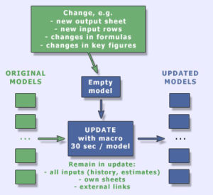
In practise the process goes so that first Valuatum or broker makes the changes to a file called empty model. The change can be e.g. a new output sheet or change in a formula anywhere in the model.

Then someone starts a macro and selects all the models that will be updated. The beginning of the process can be delayed e.g. to the late night so that no analyst work will be interrupted. When the macro finishes, all the selected models include the latest changes.

During the process the macro copies all the input values (history and estimates) and own sheets to the selected empty model.

How to make changes to the Excel model?

The answer depends on what you would like to change:

1. Output-sheets: update empty model, run conversion and inform Valuatum afterwards.
2. Own input sheets (not I-main or I-divQ): just go ahead, you can do anything you like with them.
3. I-main and I-divQ, I would like to input formulas instead of figures: just go ahead with cells in blue font and own areas; formulas and even external links are allowed.
4. I-main and I-divQ, other changes like new rows etc: contact Valuatum, we will do it for you.

The chart macro in the Excel model – how to use the chart efficiently

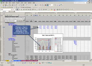
In the Excel model, you can easily display the figures in the table graphically with a ready-made chart macro. In the chart, figures are readily interpretable, and it may be easier to change the figures, as you can see how your estimate relate graphically to historical quarter figures.

Though, the chart macro is easy to use and you probably need only information how to get started i.e. where to find that macro (1 Running the macro), here are also some other instructions and some hints on how to deal with the graphs.

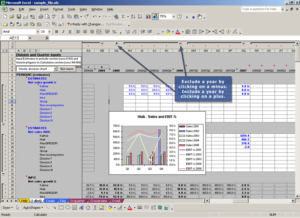
1. Running the chart macro Go to the I-divQ sheet and select the Create division chart at the macro menu and click on Run macro button.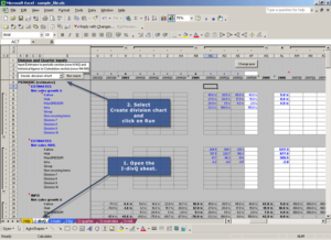

2. Choosing division and chart type Choose a division you want make the chart of and the chart type. Click then OK.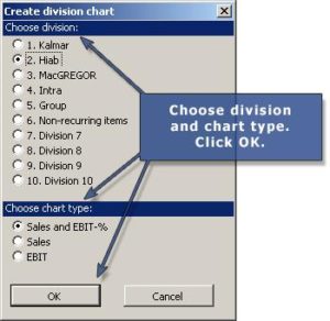

 

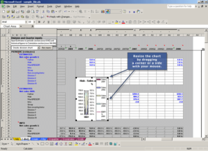
3. Moving the chart A chart of the selected division and type is opened. You can move the chart, and the possible toolbar, by dragging them with your mouse.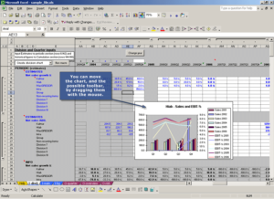

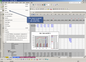
4. Excluding and including years in the chart If you want to exclude one or more years from the chart, just click on the minus sign on top of the corresponding year. Including of a year is done similarly, this time just click on the plus sign of the corresponding year.

5. Resizing the chart Especially, when excluding a year from the chart, the chart may become too small to be clear anymore. To fix this, just resize the chart by dragging one of the corners or sides with mouse.

6. Seeing the figure changes in the chart Try the chart now and change one of the changeable figures in the table. Remember to change the figures of the division that is in the chart! If the chart is on top of the division’s figures, move it somewhere else (see the point 3). Also, notice that the chart is not updated before you verify the change in a cell by pressing the Enter on the keyboard or selecting another cell.

7. Saving the chart To save the chart, you do not have to do anything extra; the chart is saved as you save the excel model, and is usable when you open the file next time. Of course it is also very easy to create the charts again so you can also remove the charts.

8. Removing the chart You can also remove the chart. Remove the chart by choosing the chart and pressing the Delete button on the keyboard. You can easily create a chart again by following these instructions.

How to change year in the Excel model?

Automatic year-change function

As the fiscal year results are reported and thus current year changes into history, the valuation models have typically to be changed. New current year has to be estimated in detail and links have to be changed to output sheets.

In Valuatum Model this complicated process can be done with only one click. Every model includes a “YearChange” macro that does all the necessary actions. The running of this macro takes about 10 seconds and all the analyst has to do is press a button.

Changing year in practise

Please follow these instructions, when you fill in Q4 results:

1. Insert “x” to the cell AF4 in I-divQ (the current year’s latest quarter).
2. Fill cumulative Q4 net sales, ebit and income statement to the I-divQ sheet.
3. In I-main enter the actualized balance sheet.
4. Update the cells in blue font also to the I-main income statement.
5. Go back to I-divQ and enter new quarter estimates: net sales, EBIT and income statement – if you have not already done it before. (If the quarter estimates are blank, then current year net sales growth becomes 0% after year change.)
6. Make a backup copy of the file.
7. Press ‘Change year’ button.

Now the macro runs a few seconds and when it has finished, it will give a message box. Do the following things after the macro:

1. Enter new estimates, especially to the I-divQ sheet, where macro has copied the Y+3 values from I-main (Y+0 means the current year). If you do not yet have the quarter estimates for the new current year, please make them too.
2. Check that the model looks mainly ok. If there are errors in interest expenses, run the FixInterestExpenses macro.
3. In Shares and dividends section update the actualized share information.

How to start new division of end existing one?

Sometimes division structure changes. The most common cases are that company buys a new business group or sells an existing one. Another case might be such that company starts to report more detailed. Then you have to start new (detailed) divisions and end the current group division.

Start new division

You can start a new division simply by writing a new division name and filling history data or estimates for it.
Just remember that you cannot use net sales growth % as an estimate parameter during the first year. For example if your growth estimate would be 5% then the absolute estimate would become: 1.05 x 0 = 0. So, use absolute net sales in first year.

End old division

Ending a division does not require anything. Just stop filling new history data and estimates for the division. However, keep the division name as long as there exists values for this division in history.

Circular reference problem

When you open a model, you may see the following warning message (click picture for a larger image):

Or while using the model, you may notice that the following tool set has appeared:

Both refer to circular reference which is caused by the loop that exists in the model between income statement and balance sheet. In order to solve the problem do the following:

1.    If it still exists, click ‘Cancel’ to the warning message (if you accidentally clicked Ok, Excel help opens; you can close it).
2.    Choose from the menu: Tools – Options – Calculation.
3.    Check the iteration box.
4.    Set maximum iterations e.g. 10 and maximum change 0.001.
5.    Click Ok.

If you feel that the calculation gets slow, decrease the amount of maximum iterations. The bigger the number, the more accurately the model calculates, but also requires more calculation power from your computer.

I have to change black output cell even though it is not allowed

Sometimes you may think that you should override a formula in a cell with black font, even though you know that the rules deny it. The answer to this kind of problem is that there is always an input cell that you can use. Here are some examples:

Net sales or EBIT info fields in I-divQ sheet

You do not ever have to change info fields in I-divQ sheet. If the quarter in question has actualized, the cells get their values from cumulative figures. If it is an estimate quarter, the cells use estimate fields. So the info fields are output cells that tell you the actual periodic figure, either based on cumulative or estimate numbers.

Current year balance sheet

When the company reports interim results, you will get new information about the balance sheet. Some parameters (e.g. Other intangible assets) you can change directly since they are input parameters in the balance sheet. However, some others are output parameters (e.g. Inventories). In the latter case do not still override the formula but adjust the corresponding estimate parameter (Inventories / Net sales %) instead, if needed.

Goodwill (in balance sheet)

If the company’s goodwill has changed during the current year (or will change in the future) in a way that cannot be explained with previous year goodwill and goodwill amortization, use the field Additional goodwill in estimate parameters.

Any other

The cases above are just examples describing that there is always a way to use input cells. If you cannot figure out how to do it, please do not hesitate to ask from us.

How much history data should I fill at minimum?

This question can be split to two:

1. What should I fill so that the model would be meaningful for other users?

It is hard to draw any specific guidelines here. Basically: the more historic data, the better. However, often the company has changed its structure so dramatically that long history data loses its meaning.

If any dramatic changes has not happened, we would recommend that every company would have at least two years history data as complete: divisional (if company reports divisions) and quarterly net sales and EBIT figures. Furthermore more rough (income statement and balance sheet) historic data should be for additional two years. So, altogether 4-5 years of historic data makes a decent model.

2. What should I fill in order to get model work fluently?

This means that you need a certain amount of data in order to get model work. This is what you must fill any case:

I-divQ sheet

• Division names – At least one division (names as ‘Group’ for example)
• Latest actualized current year quarter – Mark with ‘x’ to row 4
• Latest actualized income statement to cumulative values section
• Fill at least cumulative Q4
• Latest actualized current year quarter to cumulative values section – Not needed if Q1 not actualized
• Current year (Y+0) estimates in quarter level
• Net sales and EBIT (either relative or absolute)
• Year Y+1…Y+3 estimates in full-year level
• Net sales and EBIT (either relative or absolute)

I-main sheet

• The last estimate year (as terminal values)
• Net sales growth and EBIT-%
• Latest actualized balance sheet
• No of shares for current year

How to set value for Tangible assets / net sales %?

How to choose percentage value?

Normally companies need certain amount of tangible assets relative to their turnover. In many industries this proportion is quite constant in the long-run. For example a pulp & paper company might have had fixed assets about 85% of its sales and the proportion has alternated between 81% and 89% for the past ten years.

Simplified this means that the company needs to have a paper machine worth 850 mEUR in order to generate 1000 mEUR sales in one year. Thereby it is very unlikely that the proportion of fixed (tangible) assets would change much relative to sales either in the future. Therefore it is quite logical basis for the estimates that the relation between tangible assets and net sales would remain roughly at the same level also in the future.

Estimates in Valuatum Excel model

In Valuatum Excel model Tangible assets / Net sales are estimates in I-main sheet in section Balance sheet parameters. There you can see what it has been in the history and based on this you can make the estimates for the future. If you have not estimated investments with tangible assets in absolute terms, the Tangible assets / Net sales parameter will adjust the investments automatically.

Differences inside of industry

Often the Tangible assets / Net sales ratio is rather constant even inside a certain industry, so competitors would have pretty similar relation between tangible assets and sales. Of course it is normal to have some differences inside the same industry. Some other pulp & paper company might have e.g. proportionally bigger share of certain product types (like: fine papers, tissue papers etc.) and the different products tie capital differently in production assets.

Furthermore different companies might have different philosophy in these issues and therefore two companies with exactly same businesses might have different “asset turnover”. Others tend to use their old machinery as long as possible and others tend to keep their production facility very modern. Thus the latter group might have more efficient production capacity and also smaller variable costs but higher depreciation percentage.

Fine tuning

As you have set the parameter (Tangible asset / Net sales) roughly at the right level, you can (and often also should) do some alteration to either this parameter or directly to investments. It is often so that at least current year values are easier to estimate directly with absolute investments as we often know what kind of investment plans the company has for the current year.

If you estimate only with the Tangible asset / Net sales parameter, you should also take into account cyclical factors (capacity utilisation is different over the cycle and it affects Tangible asset / Net sales) and possible changes in group structure (relative share of certain business in the group might be changing).

Adjustments to stock splits and issues

Stock splits and issues change the number of shares outstanding and, thus, make it unsuitable to compare company valuation items (e.g. EPS) before and after the stock split or issue. Hence, in order to make comparisons meaningful, the number of shares before the split or issue has to be adjusted to take into account the changed number of shares in the future year.

Reason for these steps and the order they should be done is that the share price is updated by the system every night. If you adjust the number of shares and leave the share price to be updated by the system, the Market Cap increases drastically at first (because of the old share price and increased number of shares) just to fall at the time the system updates the share price to be split-adjusted.

There are two steps you need to take to make required adjustments:

First, go to the Admin-page, enter a Tickers & Share Price and choose the ticker and click Modify. Change the new share price and click Update.

After updating the split-adjusted share price, you can go to make the following adjustments into your excel-model.

The adjustment is conducted with an item called Stock issue multiple as follows:

• Enter a multiple to the Splits and stock issues row in the split or issue year. The multiple is determined as follows:
  • For e.g. 1:4 splits, the multiple is 4
  • For stock issues, the multiple is the ratio of the pre-issue share price and the post-issue share price (calculator)
• Compute the Stock issue multiple (for pre-split or -issue years) by multiplying the following year´s Splits and stock issues multiple with the following year’s Stock issue multiple.The next picture illustrates the adjustment process:

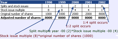
Notice that the order of these rows may vary over the time.

The adjustment has a straight effect on the following valuation items:

• Number of shares (Series I and II, diluted and average)
• Share price (Series I and II)
• Dividend per share (Series I and II)

So, in adjusting the above items to stock splits and issues, different Valuation and Per share figures can be computed in a meaningful manner.

Remember also dividend forecasts!

After these changes you probably have one more thing to fix: you probably have estimated future dividends as an absolute figure for a couple of future years. Therefore you also have to manually adjust these to reflect new situation. Of course it might be that your dividend estimates are done with payout ratio and if that is the case, then you do not have to adjust them as payout ratio estimates are of course the same before and after the split.

Reported cash flow parameters

There is no separate Cash Flow statement in the Valuatum model. Instead, cash flow is represented by the “DCF-calculation”, the area located about row 200 on the ”I-main” sheet.

By default Valuatum’s model derives cash-flow figures from the Profit & Loss statement and the Balance Sheet. While this is usually fine for the estimate years, for historical years it is very possible that derived cash flow is quite far from the cash-flow figures reported by the company. Especially large differences may be found while looking at the separate cash-flow items.

If you are not satisfied with the cash-flow figures calculated by the model, you can override them with the figures reported by the company. For that, please use the area called “Reported cash-flow parameters” which is located on the “I-main” sheet around row 300.

This area allows you to override following cash flow items:

• Change in working capital
• Taxes paid
• Cash flow from operations
• CAPEX
• Cash flow from investments
• Cash flow for the year

You can override just a few items or all of them, cash flow figures will adjust automatically. Note that there is no effect on the result of the DCF calculation (i.e. Fair Value) as only historical part of the DCF is changed. Please refer to the table below which describes how “Reported cash flow” items affect historical part of the “DCF-calculation”.

“Reported cash flow” item	Effect on historical part of  “DCF-calculation”
Change in working capital	Overrides “Change in working capital” item
Taxes paid	Overrides “Paid taxes” item
Cash flow from operations	Overrides “Operating cash flow” after following adjustments: –   net finacials +  taxes on net financials
CAPEX	Overrides “Gross capex, tangible” after following adjustments: –    Gross capex, intangible +    Acquisitions/Divestments +    Change in associates value correction
Cash flow from investments	Overrides “Change in other long-term liabilities”after following adjustments: –          Gross capex, intangible –          Gross capex, tangible +    Change in associates value correction
Cash flow for the year	Item has no effect on the “DCF-calculation” area, since DCF calculation considers only cash-flow from operations.

In order to reset default Balance Sheet and Profit & Loss driven cash flow calculation, simple delete values from the “Reported cash-flow parameters” area.

Instructions for share issue

When company does a share issue, there are two variables that affect Valuatum Excel model. First is capital increase and second is number of shares. Here are step-by-step instructions to handle rights issue in Valuatum Excel model. All the row numbers are from empty_model_552.

1. Allocate collected new capital to shareholders equity and liabilities.  We recommend you to use two different inputs, depending how company is allocating the new capital.

• The first proportion allocated to ‘share capital’ (row 155) is the proportion that is used to increase share capital
• Second proportion allocated to ‘other equity’ (row 159) is the capital reserves proportion

After increasing the equity, the model will make the balance sheet even in following order:

• Reducing debt to desired minimum level or zero
• Increasing cash

So you can change the amount of capital allocated to cash by changing the minimum level of debt (Rows 41 and 42) to match the desired level of debt. E.g. if you want all the issued capital to increase cash, adjust the minimum amount of debt to the current level. More information about how the balance sheet is made even can be found in section “How the Balance sheet is made even?”.

2. Enter the cash effect to the “Manual cash flow adjustments” (row 91). Entering the cash flow manually adjusts the DCF-calculation.

3. Adjust the number of shares. You need to input the total year end number of shares to the ‘No of shares y.e.’ (row 67). And if you need to adjust the average number of share, input it to row ‘average no of shares total (dominating)’ (row 69).

4. Adjust historical figures to make years comparable. In excel model you should use the ‘Splits and stock issues multiple’ (row 74). This multiple equals pre-issue share price divided by post-issue share price. You may find more information about splits and share issues and a multiple calculator from the instructions under “Adjustments to stock splits and issues”.

Estimating EBITDA instead of EBIT

Normally estimating in the Valuatum model is based on parameter EBIT. For some industries (e.g. telecommunications) it’s typical to report EBITDA figures for divisions and therefore it’s natural to use EBITDA in divisional estimates instead of EBIT.

Below there are instructions on how to use EBITDA in excel-model (Note: This feature exists only on Empty model versions from 561):

Step 1. Change the estimate parameter to EBITDA in I-divq –sheet Cell W2.

It’s also possible to use EBITA as estimate parameter.

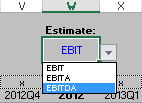
Step 2. Insert divisions In I-divq –sheet cells E9:E18

You can type EBITDA after the division name to avoid misunderstandings, if the figure is shown under EBIT somewhere in the system (e.g. template). After naming the company’s divisions, insert “Depreciation & Amortization” as a last division.

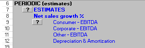
Step 3. Use EBITDA in estimates and insert whole group’s D&A for the last division

After inputting whole group’s depreciation & amortization for the last division (negative value), the divisions total equals to EBIT, even though you use EBITDA figures for divisions.

After these 3 steps you can estimate using EBITDA figures, and everything else in the model works exactly like before. Notice that depreciations & amortizations should also be inserted in the income statement (Rows 134 – 136 for estimates and rows 194 – 196 for actualized years).

Estimate period length

The default length of estimate period is 10 years but it is possible to choose any number of years between 10 and 50 in the Excel-model.

10 estimate years are usually enough, but for example in the mining industry there can be a company that has only one mine which produces output for 30 years and then it’s worthless. In such a case it’s important that the estimate period is 30 years and after that the company doesn’t generate any cash flow. With only 10 year estimate period an analyst couldn’t create a decent DCF valuation of the company. For more information about DCF valuation, see “DCF-Valuation” on page Wacc & Valuation.

How to increase the length of estimate period

In Excel-model click “Options” in I-main –sheet and choose “Define estimate period”. From there you can define the new length and after pressing “Continue” the model will add new columns to match the chosen length. Please notice that the length has to be between 10 and 50 years.

How to use estimate period less than 10 years

The minimum estimate period in the Excel-model is 10 years. However, if you want to estimate shorter period (e.g. only 5 years) you can modify your model in a way that you actually have to estimate only 5 years period, and forthcoming years work like terminal years.

You can do this by setting all the growth ratios, margins and other parameters on the I-main sheet for the estimate years 6-10 to equal the corresponding values of the estimates year 5. Then you don’t have to estimate any further than next five years, and you’ll get the same result as the model would have only five years estimate period.

Unable to run the “Year change” macro

If your “Change year” macro gives a runtime error or you end up with reference error(s) (“=#REF!”) on your “I-main” sheet, you need to remove the references to previous years, before running the macro.

References to previous years

The “Change year” macro deletes the values of the oldest time period and moves all time periods one step towards the oldest.  This removal of the oldest time period causes a problem if you are referencing to these deleted values in your becoming years.

Removing unwanted references

You can avoid the errors by clearing the references to the oldest time period before running the “Change year” macro.

Removing the references:

1. Go to your “I-main” sheet.
2.  Look for references to the previous year in the cells of the second oldest time period.
   
3. When you find a cell, which is referencing to the corresponding cell of the previous year, just copy the cell.
4. Paste the cell in itself by using the paste as “Value” option in Excel. This keeps the value, but removes the reference.
   
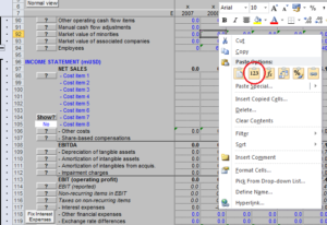
5. Repeat this to all the cells which have a reference to the oldest time period.
6. When there are no references left to the first time period, the removal of this column will not affect the remaining figures.

For example if your columns D and E include the figures of two successive years and you are going to run the “Change year” macro:

1. Check the column E for any references to column C.
2. If you find a reference for example to cell D92 in the cell E92, just copy the E92 and paste it as a values into E92 itself.
3. The values in neither E nor D 92 should change, but E92 will not have a reference to D92 left anymore.

Tips

• To avoid the caused problem, try not to use references to the previous year.
• Do the previous steps to other columns as well, not just the second oldest time period. This way you will avoid the problem in the future.

Application- or object-defined error

If you got the following warning from Excel, this

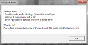
The problem is often caused by two or several named ranges that has the same name. This is often the result of some kind of copying between different models.

Try to follow the steps below to fix the problem:

1. In Excel, open the Formulas-tab and go to “Name Manager”.
2. Sort the names by the “Refers To” –column, by clicking on the bar.
3. All the external references should now be on the top of the list or at least sequentially. External references contain a reference to another  file, such as [Second_workbook.xls]
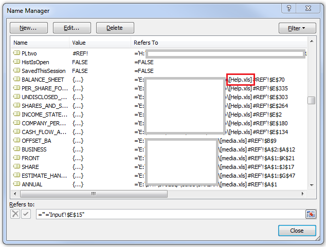
4. Select all names containing external references and click “Delete”.
5. Re-run the macro that caused the error, and it should now be working.

Forecasting Depreciations & Amortization

There are two ways to enter amortization the Valuatum system: user can either enter quarterly forecasts or enter amortization %. There is no need to use both methods. User should choose which one suits better for the current situation and go with it. The use of both of the methods might cause some errors and therefore we do not recommend it.

Quarterly amortization

If user decides to enter quarterly amortization of intangible assets, the system will calculate the sum of these inputs and uses the inputs.

Amoritization%

In the Valuatum system, the annual amortization is calculated from the amortization % and last year’s other intangible rights. E.g. user set amortization % to be 33% and other intangible rights in 2015 were 15.5. Thus, amortization in 2016 will be 5.17.